- (*)
Median for minimizing L-1 norm:
For a given vector x = [x1, ... xn], prove that the median of elements in x can minimize the following objective function based on L-1 norm:
Median of x = arg minu S|xi-u| - (*)
Mean for minimizing L-2 norm:
For a given vector x= [x1, ... xn], prove that the mean of elements in x can minimize the following objective function based on L-2 norm:
Mean of x = arg min u S(xi-u)2 - (**)
Function for for note segmentation:
Write an m-file function myPv2note.m for note segmentation, with the following usage:
note = myPv2note(pitchVec, timeStep, pitchTh, minNoteDuration) where- pitchVec: The input pitch vector
- timeStep: The time for each pitch point
- pitchTh: Pitch threshold for creating a new note
- minNoteDuration: The minimum duration of a note
- note: The output note vector of the format [pitch, duration, pitch, duration, ...], where the units for pitch and duration are semitone and second, respectively.
- Please use the pv file of "Happy Birthday" for note segmentation. You can hear the original wave clip and the corresponding midi file.
- Please use the pv file of "Twinkle Twinkle Little Star" for note segmentation. You can hear the original wave clip and the corresponding midi file.
- You can start with the pv2note.m in the SAP Toolbox, which do not take rests into consideration.
- You can use pvPlay.m to play the pitch vector, and use notePlay.m to play the output notes.
- (**)
Function for linear scaling:
Pleae write an m-file function mylinearScaling4qbsh.m for linear scaling, with the following usage:
[minDist, bestPitch, allDist] = myLinearScaling4qbsh(queryPitch, dbPitch, lowerRatio, upperRatio, resolution, distanceType) where- queryPitch: the pitch vector of the input query. This is the vector to be expanded or contracted.
- dbPitch: a pitch vector in the song database
- lowerRatio: lower ratio for scaling
- upperRatio: upper ratio for scaling
- resolution: total number of scaling (contraction or expansion)
- distanceType: distnace type, 1 for L1 norm, 2 for L2 norm.
- minDist: mininum distance of the linear scaling
- bestPitch: the pitch vector of the input query after scaling (expansion or contraction) and transposition that can achieve the mininum distance
- allDist: all distances of linear scaling
- If the expanded queryPitch is greater than the length of dbPitch, then stop doing linear scaling.
- For L-1 norm, we need to do median justification. For L-2 norm, we need to do mean justification.
- You need to perform distance normalization.
- You can assume the input vectors do not contain rests.
- Please run this example, but replace linScalingMex with myLinearScaling4qbsh to see if you can get the same result. (Note that in order to save computation, "linScalingMex" does not take the squar root when computing L-2 norm.)
- Use your function in the programming contest of QBSH to see if you can achieve the same recognition rate.
... sf=linspace(lowerRatio, upperRatio, resolution); queryLen=length(queryPitch); for i=1:resolution Find the length of the scaled query (scaledQuery) Get out of the loop if scaledQuery is longer than dbPitch Obtain scaledQuery by interp1 Find the difference (diffPitch) between scaledQuery and dbPitch Find the median of diffPitch allDist(i)=norm(diffPitch-median, distanceType)/length(scaledQuery); scaledTransposedQuery{i}=... end [minDist, minIndex]=min(allDist); bestPitch=scaledTransposedQuery{minIndex}; ... Hint: You can use "interp1" for interpolation, "median" for computing median, "mean" for computing mean, "norm" for computing Lp norm. If you do not know how to use "interp1", the following is an example:
- (***)
Linear scaling for chart detection:
In this exercise, you need to write a function for chart detection in technical analysis of FinTech. Your function should look like this:
[distance, queryTransformed]=linScaling4chart(query, dbVec, sfMin, sfMax, sfCount, alphaMin); where- inputs:
- query: Chart pattern to be detected
- dbVec: Vector in the database, where the given query is to be found
- sfMin: Min. of the scaling factor
- sfMax: Max. of the scaling factor
- sfCount: Count of the scaling factors (which is equal to the no. of contractions/expansions of the query)
- alphaMin: Min. of alpha (Please check out the code template for more details.)
- outputs:
- distance: Normalized distance
- queryTransformed: The best transformed query (which is as close as possible to a portion in dbVec)
And here is a test example:
- inputs:
- (***)
Function for type-3 DTW:
Please write a m-file function myDtw3.m for type-3 DTW, with the usage:
[minDist, dtwPath, dtwTable] = myDtw3(vec1, vec2) You can start from the following skeleton:To test your function:
- Try this example, but replace dtw3mex by myDtw3 to see if you can obtain the same result.
- Use your function in the programming contest of QBSH, with 1 key transposition. What is the recognition rate?
- Use your function in the programming contest of QBSH, with 5 key transpositions. What is the recognition rate?
- (***)
Methods for improving type-3 DTW:
Write a m-file function myDtw3b.m for type-3 DTW, with the enhancements mentioned at the end of the section covering type-3 DTW:
- Set the range of frame numbers being mapped to each note: For instance, the duration of the frames being mapped to a note should between the range [0.5, 2] of the duration of the note. This can enhance the performance since the duration of each note is used.
- Use rests: Except for the leading and trailing rests, any rest in the query input indicates the end of the previous note and the beginning of the next note. We can use this cue for better alignment and query by singing/humming.
- Use both of the above enhancements.
- Use your function in the programming contest of QBSH, with L-1 norm and 1 key transposition. What is the three recognition rates?
- Use your function in the programming contest of QBSH, with L-1 norm and 5 key transpositions. What is the three recognition rates?
- (***)
QBSH accuracy w.r.t. LS resolutions and no. of key transpositions:
Before attempting this exercise, you should first fully understand the example program in the programming contest of QBSH. You tasks are explained next.
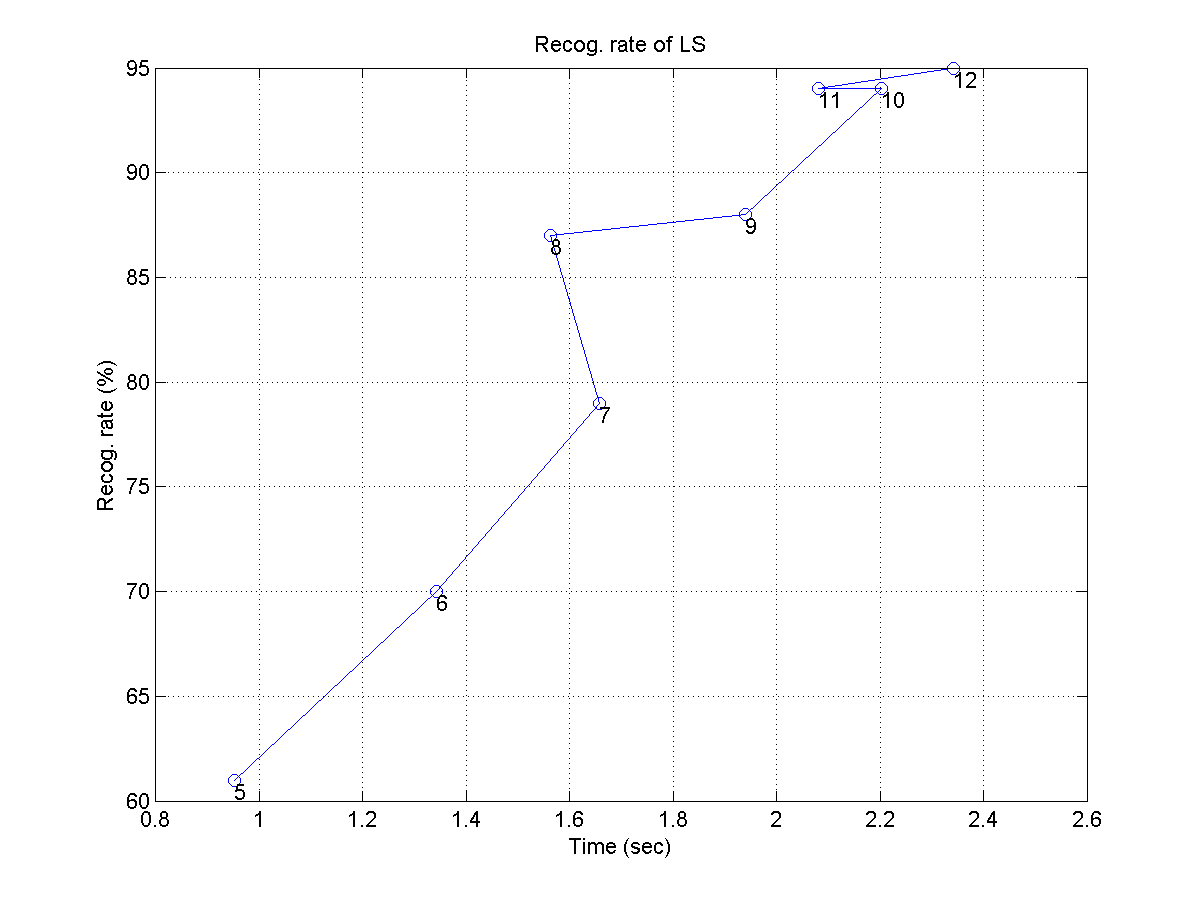
- Use linear scaling for QBSH, and plot the recognition rate as a function of the computation time, but parameterized by the resolution for linear scaling from 5 to 12. Your plot should be similar to the following one:
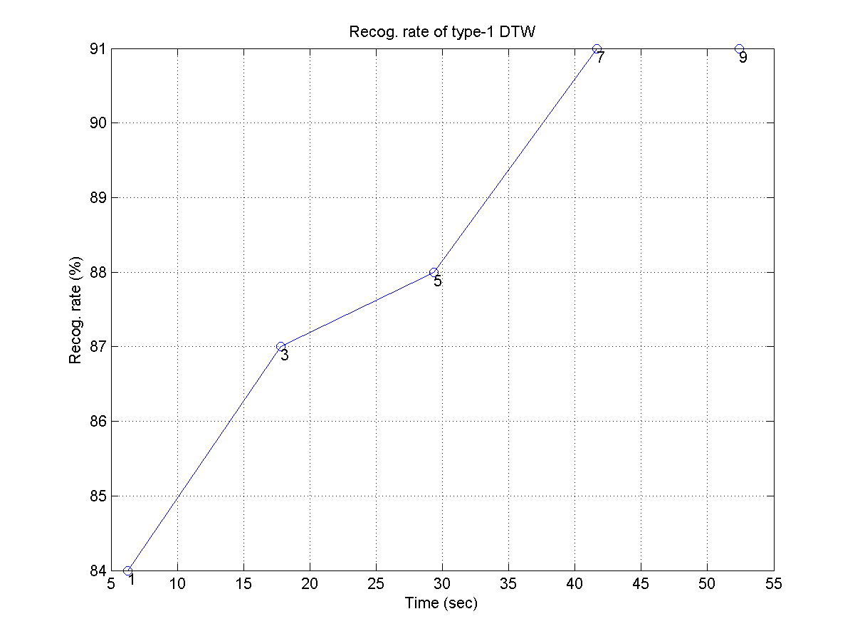
- Use type-1 DTW for QBSH, and plot the recognition rate as a function of the computation time, but parameterized by the numbers of key transposition of [1, 3, 5, 7, 9]. Your plot should be similar to the following one:
- If the computing time is too long, you can use the first 100 wave files for this exercise.
- It would be easier for you to do the computation and plotting if you modify the example program in the programming contest for QBSH into a single function.
- Use linear scaling for QBSH, and plot the recognition rate as a function of the computation time, but parameterized by the resolution for linear scaling from 5 to 12. Your plot should be similar to the following one:
- (***)
QBSH accuracy w.r.t. pitch vector reduction ratio:
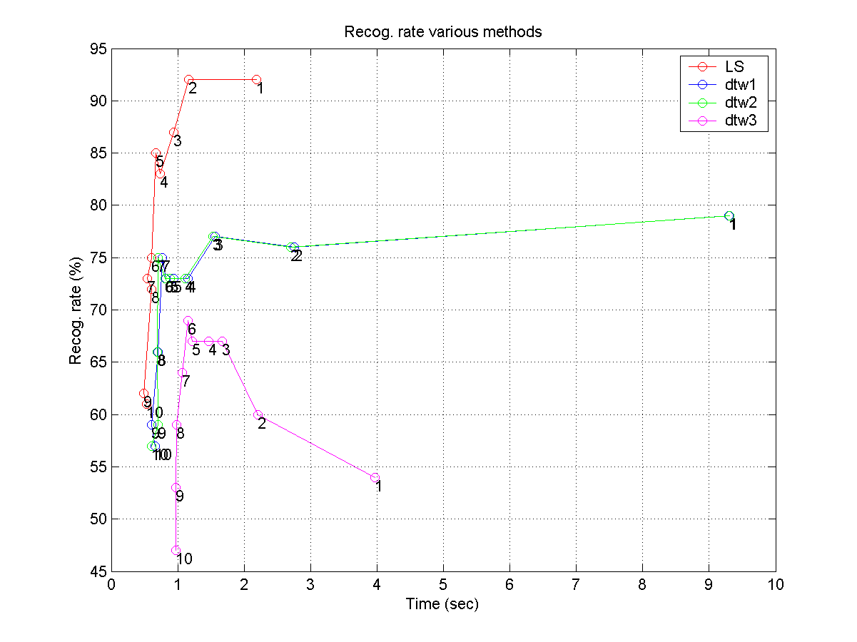
Before attempting this exercise, you should first fully understand the example program in the programming contest of QBSH. The pitch rate of our query pitch vector is fs/frameSize = 8000/256 = 31.25. If the computing time is too long, we can simply down-sample the pitch vector to reduce the size of the DTW table. In other words, we can explore the effect of PVRR (pitch vector reduction ratio) on the recognition rates of various methods. For a given value of pvrr, the pitch rate becomes 31.25/pvrr. You need to plot the recognition rates of 4 methods (LS, DTW1, DTW3, DTW3) with respect to computation time, but parameterized by PVRR which varies from 1 to 10. Your plot should be similar with the following one:
- If the computing time is too long, you can use the first 100 wave files for this exercise.
- It would be easier for you to do the computation and plotting if you modify the example program in the programming contest for QBSH into a single function.
- (***)
Creating a QBSH prototype using linear scaling:
In this exercise, you are going to write a MATLAB script to create a prototypical QBSH system. Basically, the user can sing/hum to the microphone for 8 seconds and the system can list the top-10 ranking of the retrieved songs based on their similarity to the query input. Before trying this exercise, you should download the following toolboxes and add them to your search path:
Your system should follow the following steps:
- Load the song database. This can be achieved by using
songDb=songDbRead('childSong'); You can check the contents of songDb by typingstructDispInHtml(songDb); In particular, songDb(i).track is a vector in the format of [pitch1, duration1, pitch2, duration2, ...], which specifies the melody track of the i-th song in the database, where pitch is in the unit of semitones and duration is in the unit of 1/64 seconds.Once you have loaded the songs into memory, you can play the songs by using
notePlay. For instance, if you want to play the first 30 notes of "Yankee Doodle", try the following command:notePlay(songDb(42).track(1:60), 1/64); (Remember to turn on your speakers.) If you want to see the pitch contour of the song, trynotePlot(songDb(42).track, 1/64); If you want to see the pitch contour together with the generated waveform, try:notePlay(songDb(42).track(1:60), 1/64, 1, 1) - Convert the "track" field of each song to PV (pitch vector) representation and attach the PV to a field "pv" of songDb. You can use the command
note2pv. For instance:[pv, noteStartPvIndex]=note2pv(songDb(42).track, 1/31.25, [], inf, 1); The above command will convert song 42 (Yankee Doodle) into a pitch vectorpv, with a pitch rate of 31.25. A plot will also be shown to demonstrate how the music notes are converted into PV. (Please try "help note2pv" for detailed usage.) - Do 8-second recording with fs=8000, nbits=8.
- Perform pitch tracking by using the command
ptByPf. Plot the result of pitch tracking (by supplying appropriate arguments to the command) after each recording to make sure the pitch tracking result is satisfactory. (Try "help ptByPf" for its usage and example.) - Handle rests by using the command
restHandle. - Compare the query PV to each PV in the database using
linScalingMex. (Please make sure you understand the example of linear scaling used in the text.) - Display the top-10 retrieved songs based on the LS distances.
- Load the song database. This can be achieved by using
- (***) Creating a QBSH prototype using DTW: Repeat the above exercise using DTW. Make sure to explain to the TA how you perform key transposition.
- (***) Programming contest: query by singing/humming: Please follow the link for more information.
Audio Signal Processing and Recognition (音訊處理與辨識)
